How to Properly Measure Risk

The views presented here do not necessarily represent those of Advisor Perspectives.

In a 2020 Advisor Perspectives article, I wrote:

A few years ago I attended a conference at which most of the talks were about finance. Of course, the topic of risk was central to many of them.

After a talk by a luncheon speaker, there were audience questions and comments. One of the attendees, John Kay, himself a conference speaker, rose and gave his view that risk was defined not by volatility but through “narratives” — of which I will speak later.

Immediately after lunch I attended one of the afternoon’s parallel sessions. It was given by a finance professor and one of his graduate students.

The professor began by saying, “John Kay says risk is defined by narratives.” He then held his hands up, palms upward, shrugged and said, “What can you do with that?”

What he meant, I soon learned, was, “How can you make use of that observation to develop a long series of complicated-looking mathematical formulas in a PowerPoint presentation?”

Narratives can’t be expressed in mathematical formulas. But in this professor’s view — and the view of much of the academic finance field — you’re “doing something” only if you’re developing a series of complicated-looking mathematical formulas.

Narratives in the Definition of Risk

In their book Radical Uncertainty, as I wrote in that article, British economists John Kay and Mervyn King define the role of narratives this way:

“Risk,” they say, “is a failure of a projected narrative, derived from real-life expectations, to unfold as envisaged.”

Insurance, for example — a pre-eminent risk-mitigation measure — “is based not on calculations of expected value, but on the desire to protect the reference narrative of the insured.”

“The key to managing risk,” the authors go on to say, “is the identification of reference narratives which have these properties of robustness and resilience.”

The Investment Reference Narrative

In most cases, the reference narrative that an investor desires to protect is one in which the investor has access to desired cash flows at desired future times. The goal isn’t simply to build up wealth, though some investment strategy approaches might make you think it is.

Rather, the goal is — or should be — to invest for a purpose. That purpose is to have access to desired amounts of cash at future times when you need them — that is, when your reference narrative says you will need them.

The retirement reference narrative is the paradigmatic example of an investment narrative. An investing couple, for example, invests to have access to sufficient cash flows in the future. Risk is the risk of failing to achieve this. That is, it’s the risk of running out of money while attempting to withdraw those cash flows.

This Risk Can Be Quantified

There is a way to quantify this risk. It is not volatility.

I wrote a computer program to do it. Below, I describe the program and the data it uses. Then I specify a set of assumptions I fed into the program to obtain results for the case of a couple who invest for retirement. Next, I display the results of running the program for those assumptions and variations on them.

I then list the conclusions reached from using the program and its results. After that, I explore the unsettling implications. Finally, I describe possible improvements to the data the program uses and potential expansions of its use.

The Data the Program Uses

Aswath Damodaran, a finance professor at the Stern School of Business, maintains a database of annual returns on U.S. stocks (S&P 500), Baa Corporate Bonds, 3-month U.S. Treasury Bills, and inflation. Annual returns and inflation currently run for 98 full years, from 1928 through 2025.

I corrected the returns for inflation so that all dollar amounts used in the program are in real dollars.

The Program

The program calculates the probability that an investor will run out of money while attempting to withdraw the cash flows specified in the investor’s reference narrative. In this version of the program’s application, the “investor” is actually a couple investing for retirement. The couple will invest until retirement age. They will make annual withdrawals until the second survivor dies. (I used the female actuarial tables for convenience, on the assumption that the female is likely to be the second survivor. Using joint and survivor tables would be slightly better.)

The Example: A Couple’s Reference Narrative

Let us assume the couple are the same age and they begin investing when they are both 25, starting with no assets. The initial assumption is that they contribute $3,000 to their investment fund in the first year, then increase it by 5% each year after that until a final contribution at age 65.

After age 65, they attempt to withdraw $50,000 each year for as long as one of them survives. Their initial reference narrative specifies a bequest at the death of the second survivor of $100,000.

We assume the couple invests in low-cost index funds with a management fee of five basis points, or 0.05%. These assumptions are all inputs to the program and can be altered. All dollar amounts are in real dollars.

The Method of Calculating the Probability of Running Out of Money

For this specific example, the number of years of accumulation before retirement is 41 (ages 25 to 65). If the couple potentially lives to age 100 the years of decumulation are 35, or until the death of the second survivor if earlier. Hence, the total number of years of accumulation and potential decumulation is 41 plus 35, or 76.

Within the 98 years of Damodaran’s data (1928 through 2025) there are 23 contiguous 76-year sequences, from 1928–2003 through 1950–2025. The initial approach is to run the couple’s 76 accumulation and decumulation years through each of these 23 sequences of returns. Let us say, for example, that in just 2 of those 23 sequences, the couple runs out of money while trying to make their desired withdrawals. That is a failure probability of 2/23 or 8.7%.

But 23 sequences are not sufficient for a meaningful estimate of the probability. An additional technique must be used. That technique is to take those 98 years of stock and bond returns and randomly permute them — shuffle their sequences of returns. This can provide any number of additional sequences of 76 accumulation and decumulation years.

This is similar to a technique used by Eugene Fama and Kenneth French in their 2009 article “Luck Versus Skill in the Cross Section of Mutual Fund Returns.” It has been applied in many other studies as well. Like a random walk, this technique assumes that sequential investment returns are statistically independent of each other, an assumption that bears out well when the historical evidence is examined.

This technique’s advantage over the usual Monte Carlo simulation approach is that the probability distribution of returns is the one that is observed in actual historical returns data, rather than the typical Monte Carlo assumption of a normal (actually, lognormal) distribution of returns. This deals with the “fat tails” objection to such simulation techniques.

When this method is used, the couple’s inputs can be run through any number of simulations to obtain a robust probability of failure to protect their reference narrative.

Results

Table 1 shows results for a variety of assumptions.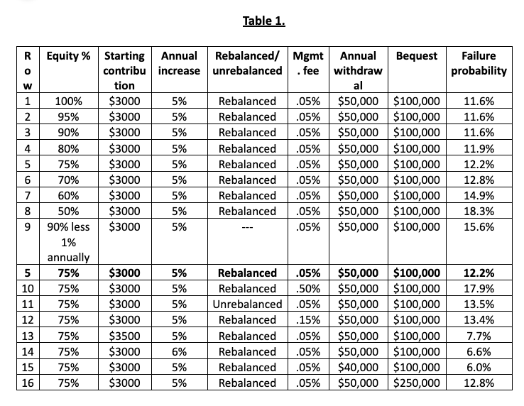

Conclusions Reached from These Results

These are the conclusions to be reached from the results in Table 1.

For Rows 1–9, the risk of failure to achieve reference narrative increases with declining equity allocation while

Probability of failure increases at a steeper rate as equity allocation declines.
Probability of failure does not vary greatly when the equity percentage is above 75%.
An age-based strategy of 90% initial equity declining 1% annually offers no improvement.

Suppose that the investing couple — while they are convinced that a higher-equity allocation is better than a lower one — is a little skittish about equities offering no firm promise of later value and about volatility. Therefore, they choose 75% equity for a failure probability of 12.2%, as compared to the slightly lower failure probability of 11.6% for 90–100% allocation.

Rows 10–16 of Table 1 alter other assumptions while maintaining the 75% equity allocation. Line 5, the base case, is repeated directly above lines 10 to 16 for easy comparison. Results are as follows:

Compare rows 5 and 10: An increase in the management fee from 0.05% to 0.50% increases failure probability from 12.2% to 17.9%.
Compare rows 5, 11, and 12: Rebalancing reduces risk slightly over not rebalancing, but not enough to warrant paying more than 10 basis points annually for rebalancing.
Compare rows 5 and 13: Increasing the initial contribution from $3,000 to $3,500 while maintaining 5% subsequent annual increases reduces the failure probability from 12.2% to 7.7%.
Compare rows 5 and 14: Maintaining the initial contribution at $3,000 but changing the subsequent increase rate to 6% annually reduces the failure probability from 12.2% to 6.6%.
Compare rows 5 and 15: Reducing the couple’s aspiration in their reference narrative from $50,000 annually to $40,000 annually reduces the failure probability from 12.2% to 6.0%.
Compare rows 5 and 16: Increasing the desired bequest by 150%, from $100,000 to $250,000, only increases the failure probability from 12.2% to 12.8%.

Implications of These Results

Almost every alteration to the assumptions has a greater impact on risk than asset allocation.

None of these conclusions would have resulted from the standard approach of a mean-variance analysis combined with an assessment of the investor’s “tolerance for risk” (i.e., volatility) leading to an asset allocation. The emphasis would have been placed instead on the two things this analysis shows are least important: asset allocation and volatility.

Possible Program Improvements & Potential Expansions of Its Use

A reasonable objection could be that the annual returns on the S&P 500 for the years 1928 to 2025 may not be representative of future returns. This near-century of data spans an unusual time in history in an unusual place, the United States. A more expansive database of equity returns is available: the Finaeon database (requires subscription). As the graph on the Finaeon equity returns web page shows, these returns have also compounded to a high level of growth over time, like the S&P 500, but over a much longer period (going back a few hundred years) and for a broader database of equities.

Program users may also have beliefs about how the future may be unlike the past — for example, that the equity premium in the future will be different from the past. If so, it is a simple matter to adjust the returns without disturbing their pattern by adding or subtracting the same increment to or from every equity return in the database.

The narrative presented in this article is uniquely suited only to the retirement scenario. (And it neglects such complications as tax-deferred accounts, etc.) Other investing narratives will be different — for example, those of pension funds or endowment funds.

Yet, in each case, the purpose of the fund is to ensure the investor’s ability to spend varying amounts of cash at distributed times in the future. To the extent that those cash flows and their timing can be estimated, however approximately, the same approach can be employed.

See more by Michael Edesess:

Economist and mathematician Michael Edesess is an adjunct professor and visiting faculty at the Hong Kong University of Science and Technology. In 2007, he authored a book about the investment services industry titled “The Big Investment Lie,” published by Berrett-Koehler. His new book, “The Three Simple Rules of Investing,” co-authored with Kwok L. Tsui, Carol Fabbri and George Peacock, was published by Berrett-Koehler in June 2014.

A message from Advisor Perspectives and VettaFi: Discover something new! Click here to register for our upcoming webcasts